'통계학 > 베이지안(Bayesian)' 카테고리의 다른 글
| Bayesian Linear Regression (0) | 2025.05.19 |
|---|
| Bayesian Linear Regression (0) | 2025.05.19 |
|---|
| Bayes Rule (0) | 2025.05.19 |
|---|
| Qualitative variables as predictors (0) | 2024.11.22 |
|---|---|
| Transformation of variables (0) | 2024.11.19 |
| 다중선형회귀 (Multiple linear regression) (0) | 2024.10.06 |
| 단순선형회귀 (Simple linear regression) (3) | 2024.09.25 |
Suppose that Z is a two-level categorical variable such that Z = A or B.
Define
$$X =
\begin{cases}
1, & \text{if } Z = A \\
0, & \text{otherwise}
\end{cases}$$
Then we can use the following regression model, $$ Y = \beta_0 + \beta_1X + \epsilon$$
Since $E(Y) = \beta_0 + \beta_1X$,
if Z = A, X = 1, $E(Y) = \beta_0 + \beta_1 = \mu_A$
if Z = B, X = 0, $E(Y) = \beta_0 = \mu_B$
Suppose that Z is a three-level categorical variable such that Z = A, B or C.
Define
$X_1 =
\begin{cases}
1, & \text{if } Z = A \\
0, & \text{otherwise}
\end{cases}$
$X_2 =
\begin{cases}
1, & \text{if } Z = B \\
0, & \text{otherwise}
\end{cases}$
Then we can use the following regression model, $$y = \beta_0 + \beta_1X_1 + \beta_2X_2 + \epsilon$$
Since $E(Y) = \beta_0 + \beta_1X_1 + \beta_2X_2$,
if Z = A, (1, 0), $E(Y) = \beta_0 + \beta_1 = \mu_A$
if Z = B, (0, 1), $E(Y) = \beta_0 + \beta_2 = \mu_B$
if Z = C, (0, 0), $E(Y) = \beta_0 = \mu_C$
Consider two categorical variables: One at 3 levels ($F_1, F_2, F_3$) and the other at 2 levels ($B_1, B_2$).
Then, the model can be written as $$Y = \beta_0 + \beta_1X_1 + \beta_2X_2 + \beta_3X_3 + \epsilon,$$
where
$$X_1 = 1\,if\,F_2\, X_1 = 0, if\,not$$
$$X_2 = 1\,if\,F_3\, X_2 = 0, if\,not$$
$$X_3 = 1\,if\,B_2\, X_3 = 0, if\,not$$
Note that $F_1$ and $B_1$ : base levels
Consider an extended model as follows:
$$Y = \beta_0 + \beta_1X_1 + \beta_2X_2 + \beta_3X_3 + \beta_4X_4 + \beta_5X_5 + \epsilon,$$
where
$$X_1 = 1\,if\,F_2\, X_1 = 0, if\,not$$
$$X_2 = 1\,if\,F_3\, X_2 = 0, if\,not$$
$$X_3 = 1\,if\,B_2\, X_3 = 0, if\,not$$
$$X_4 = X1X3, \, and\, X_5 = X_2X_3$$
Note that $F_1$ and $B_1$ : Base levels.
Since $F_2$, $B_1$, $\mu_{21} = \beta_0 + \beta_1$ then we can write $\beta_1 = \mu_{21} - \mu_{11}$.

이걸 보고 우리가 질문할 수 있는 것은 다음과 같습니다.
결론: 범주형에 대한 회귀분석을 진행할 때도 interaction을 고려해볼 수 있다는 것입니다.
| Matrix format (0) | 2025.02.18 |
|---|---|
| Transformation of variables (0) | 2024.11.19 |
| 다중선형회귀 (Multiple linear regression) (0) | 2024.10.06 |
| 단순선형회귀 (Simple linear regression) (3) | 2024.09.25 |
Transformations are applied to accomplish certain objectives such as
$$n_t = \beta_0 + \beta_1 + \epsilon_t $$
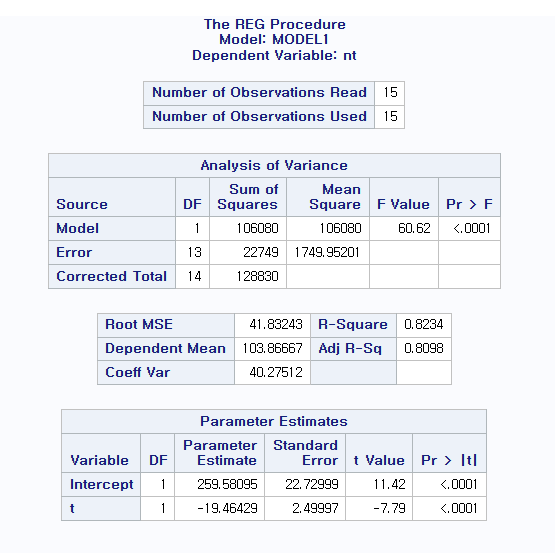

9개의 plot 중에 첫 번째 plot을 통해 Lack of fit($E(\epsilon) \neq 0$) 문제를 확인할 수 있습니다.
따라서 X 변환을 통해 이 문제를 해결해주면 좋을 듯 합니다.
그렇기에 우리가 처음 썼던 식에서 조금 변형을 해주면 다음과 같이 쓸 수 있습니다.
$$ n_t = \beta_0 + \beta_1t + \beta_2t^2 + \epsilon_t$$


그런데 첫 번째 그림에서 Lack of fit의 문제는 어느 정도 해결된 듯 보이나
unequal variance 문제가 발생하였습니다.
따라서 이 문제를 해결하기 위해 Y 변환을 고려하는 것이 좋을 듯 합니다.
생물학에서는 Bacteria deaths due to X-ray radiation 문제의 식이 따로 존재합니다.
$$n_t = n_0 e^{\alpha t}$$
따라서 이 식을 통해 다음과 같은 식을 유도할 수 있습니다.
$$logn_t = log n_0 + \alpha t$$
이 식은 $log n_t$를 Y로 생각하고 $logn_0$를 \beta_0, $\alpha t$를 $\beta_1 X$로 생각하면 선형회귀의 식으로 이해할 수 있습니다.
따라서 $$logn_t = \beta_0 + \beta_1 t + \epsilon_t$$의 값으로 fitting을 하면

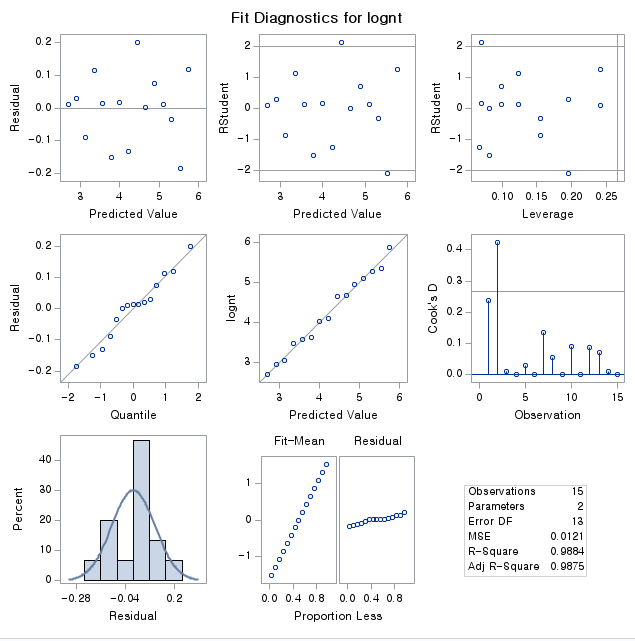
네 이렇게 해서 lack of fit과 unequal variance에 대한 문제를 해결했습니다.
3번째 그림을 통해 inferential observation을 관찰한 결과, 영향점은 없는 것으로 확인되고 있습니다.
qqplot을 통해서 Normality도 보장되고 있다는 것을 확인할 수 있습니다.
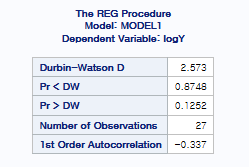
그럼 잔차의 독립성을 위해 Durbin-Watson 검정을 시행하면

다음과 같이 나옵니다.
Durbin-Watson D의 값이 2보다 크기 때문에 Pr > DW 부분의 p-value값을 통해 검정을 시행해보면
We fail to reject the null이기에 H0를 기각하지 못합니다.
그렇다고 안 좋은 게 아닙니다. 절대!
Durbin-Watson 검정은 H0를 기각하지 않아야 잔차의 독립성을 만족한다고 생각하기에
위의 값을 통해 잔차의 독립성이 만족된다는 것을 확인할 수 있습니다.
따라서 저희는 이렇게 하여 회귀분석 4가지 가정을 모두 만족시켰습니다.
또 다른 얘기를 위해 한 가지 예제를 더 들겠습니다.

여기서 R-square가 0.7759가 나왔는데 사실 field에 따라 결정계수의 높고 낮음의 기준은 다르기에 field에 따라 결정계수의 값이 높다 나쁘다가 결정됩니다.

여기서도 마찬가지로 첫 번째 그림에서 Lack of fit과 unequal variance가 의심이 됩니다.
따라서 X, Y 변환을 고려해야 합니다.
X의 제곱근을 더해주고, boxcox 변환을 통해 Y변환을 취해 줍니다.
여기서 만약 선형모형이 맞다고 생각이 들더라도 Lack of fit이 의심되면 2차를 오버피팅하는 습관은 아주 좋습니다.
어차피 선형모형이 맞다고 하면 X의 제곱의 $\hat{\beta}$ = 0 으로 나올 것이기 때문입니다.

현재 $\lamda$ = 0이 나왔기에 boxcox 변환할 때 log 변환을 취해주고 fitting을 해주면

위와 같은 결과가 나옵니다.
여기서 그림을 살펴보면 기본 4가지 가정 중 3가지는 만족하는 것으로 보입니다만,
inferential point가 2개 있는 것을 할 수 있습니다.
일단 이 결과를 바탕으로 Durbin-Watson 검정을 시행해주면
위와 같은 결과가 나오기에 We fail to reject the null 이기에 잔차의 독립성은 만족됩니다.
| Matrix format (0) | 2025.02.18 |
|---|---|
| Qualitative variables as predictors (0) | 2024.11.22 |
| 다중선형회귀 (Multiple linear regression) (0) | 2024.10.06 |
| 단순선형회귀 (Simple linear regression) (3) | 2024.09.25 |
Sales = $\beta_0$ + $\beta_1$youtube + $\beta_2$facebook + $\beta_3$newspaper + $\epsilon_i$
Q1. Write the assumptions we impose on $\epsilon$
>> $\epsilon$ ~ iid N(0, $\sigma^2$)
Q2. Using the OLS method, estimate regression coefficients.
$\hat{\beta_0}$ = 3.52667
$\hat{\beta_1}$ = 0.04576
$\hat{\beta_2}$ = 0.18853
$\hat{\beta_3}$ = -0.00104
Q3. Estimate $\sigma^2 $
4.09096
없으면 root MSE 제곱해서 답 적기($2.02261 ^ 2$)
SSE / DF = MSE
Q4. Test the overall utility of the model.
$H_0: \beta_1 = \beta_2 = \beta_3 = 0$
$H_1: \beta_j \neq 0$ for some j = 1,2,3
Let $\alpha = 0.05$
Since p-value =< 0.0001 is less than $\alpha = 0.05$, we reject $H_0$.
Thus, the overall model is useful.
Q5. Can we claim that the facebook advertising is related to sales? Justify.
$H_0: \beta_2 = 0$
$H_1: \beta_2 \neq 0$
Let $\alpha$ = 0.05.
Since p-value =< 0.0001 is less than $\alpha$ = 0.05, we reject $H_0$.
That is, we can claim that the facebook advertising is related to sales.
Q5-1. Can we claim that the newspaper advertising is related to sales? Justify.
$H_0$: $\beta_3 = 0$
$H_1$: $\beta_3 \neq 0$
Let $\alpha$ = 0.05.
Since p-value = 0.8599 is greater than $\alpha$ = 0.05, we fail to reject $H_0$.
That is, we can claim that the facebook advertising is related to sales.
This means that the newspaper advertising is not related to sales.
Q6. Compute the expected change in the sales when our spending for youtube advertisement increases by 1000달러 while the others are fixed.
45.76달러(0.04576 * 1000달러)
Q7. Compute the expected sale when we spend 1000달러 for each method of adv.
$\hat{Sale}$
45.76 + 188.53 + 3526.67 - 1.04= 3.7599 * 1000
Q7-1. Compute the expected sale when we spend 0달러 for all of adv.
x들의 값이 0일 때의 기댓값이 위의 질문에 대한 대답
$\beta_0$ => 3.52667 * 1000달러
$\beta_0$는 실제의 데이터 변수의 성질에 따라 x들의 값을 0으로 둘 수 있는지 없는지가 갈린다.
Q8. Can we argue that youtube is negatively related to the sale?
1. youtube랑 sales와 관계가 있는지부터 확인($\beta$)
2. 그러고 난 다음에 관계가 있으면 $\hat{\beta}$의 값을 신뢰할 수 있음.
왜냐하면 $\beta_1$의 값이 0이 아니라고 1번에서 결론지었기 때문에
We conclude that $\beta_1 \neq 0$.
However, since $\hat{\beta_1}$ = 0.04576 is greater than 0, we cannot argue that...
Q8-1. Can we argue that newspaper is negatively related to the sale?
We conclude that $\beta_3$ = 0. We cannot argue that ...
Q9. Compute the R-squared and interpret it.
$R^2$ = 0.8972
89.72% variability in sales can be explained
by the fitted model (with youtube, facebook, and newspaper.)
Q9-1. adj. R-squared 도 마찬가지.
| Matrix format (0) | 2025.02.18 |
|---|---|
| Qualitative variables as predictors (0) | 2024.11.22 |
| Transformation of variables (0) | 2024.11.19 |
| 단순선형회귀 (Simple linear regression) (3) | 2024.09.25 |


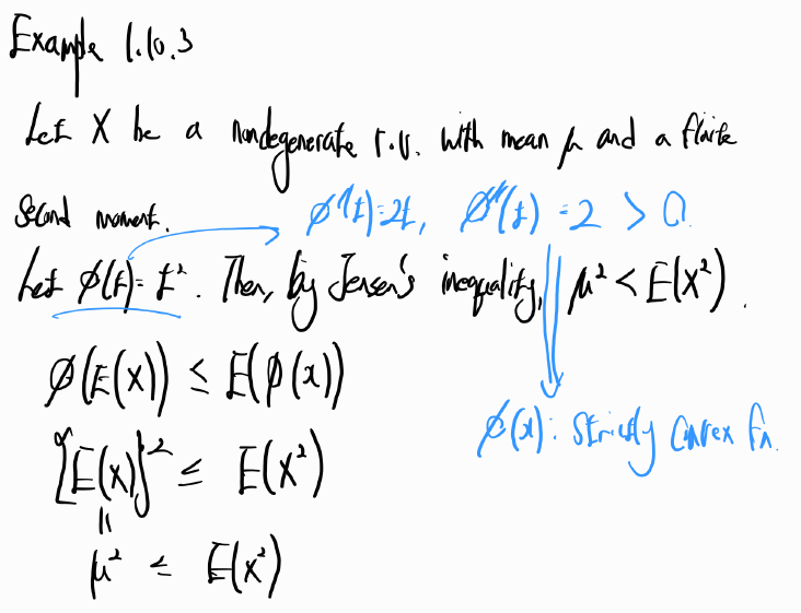
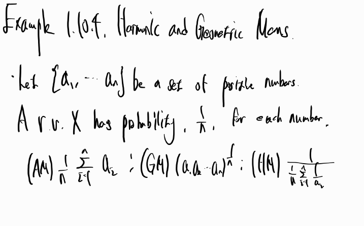
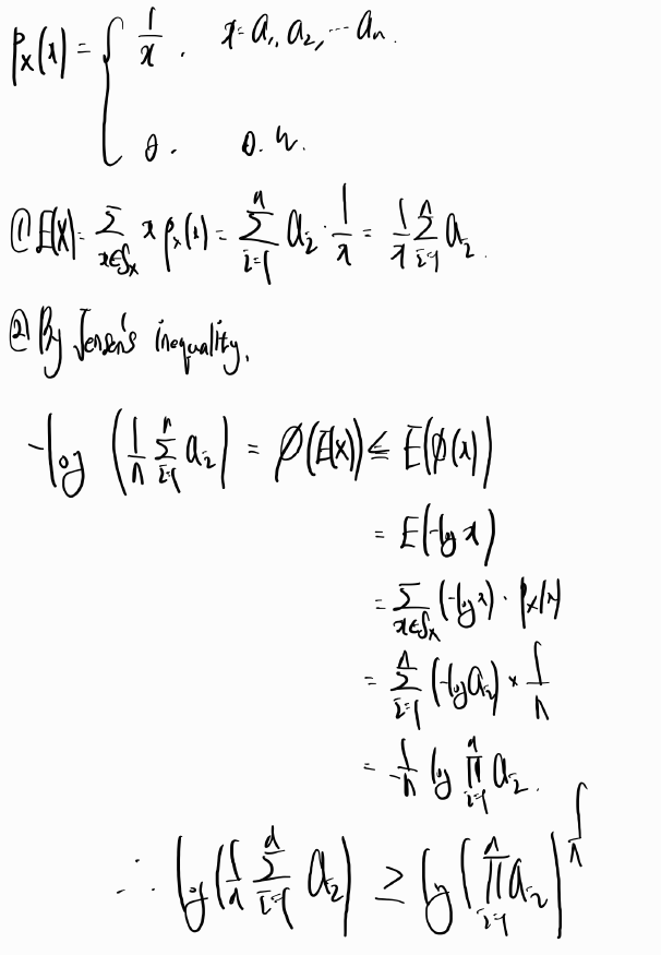
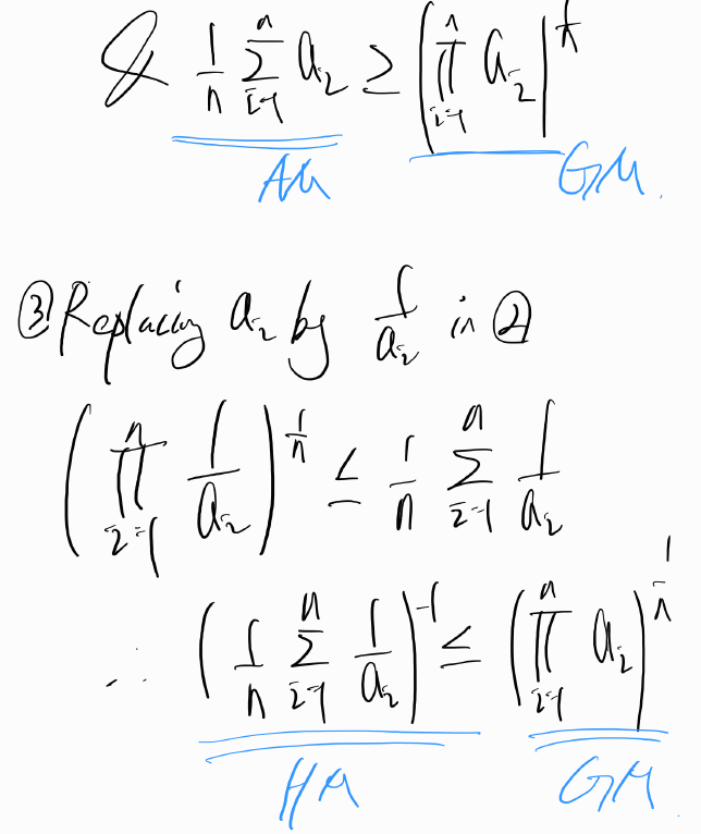
| Important inequalities (0) | 2024.10.04 |
|---|---|
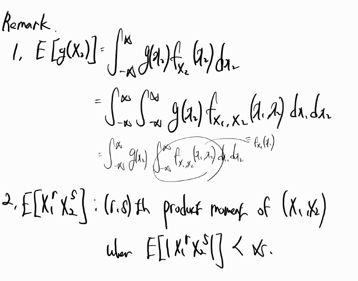
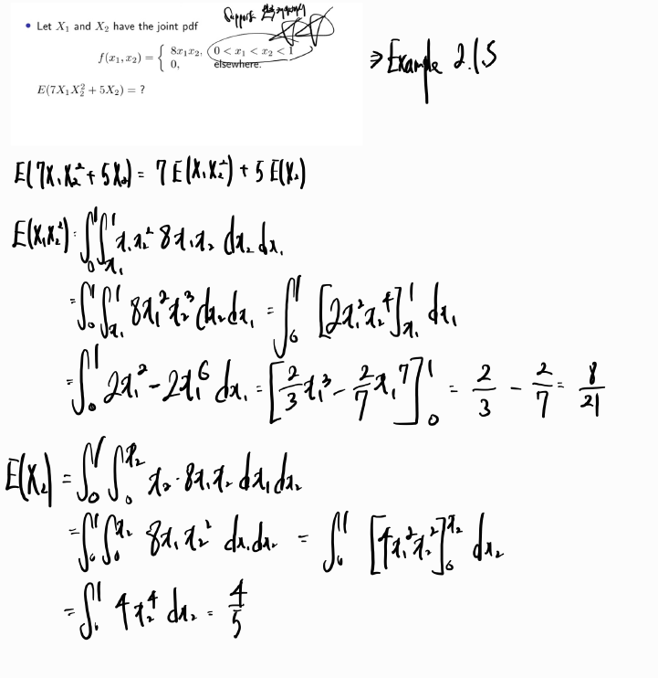
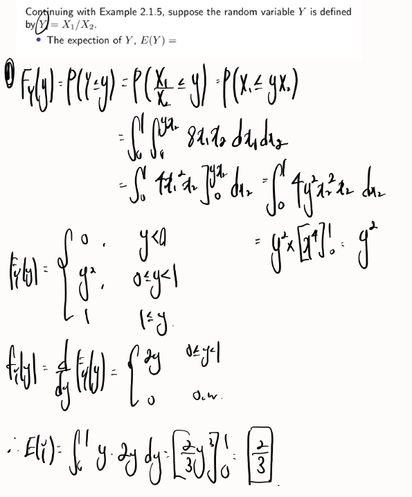
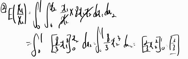
| Some special Expectations (0) | 2024.10.04 |
| Expectation of Random Variables (0) | 2024.10.04 |
| Continuous Random Variables (0) | 2024.10.04 |
| Discrete Random Variables (1) | 2024.10.04 |


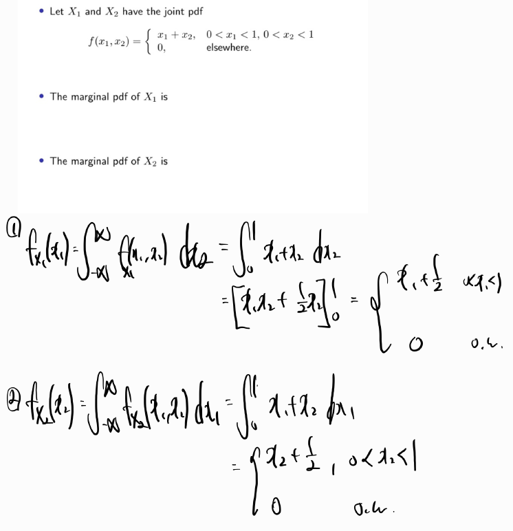
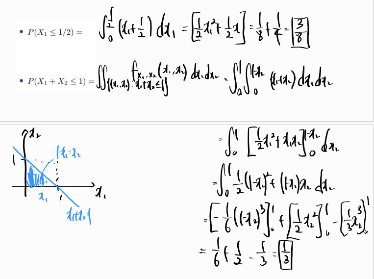
| Multivariative Distribution - Distributions of Two Random variables (0) | 2024.10.04 |
|---|---|
| Some special Expectations (0) | 2024.10.04 |
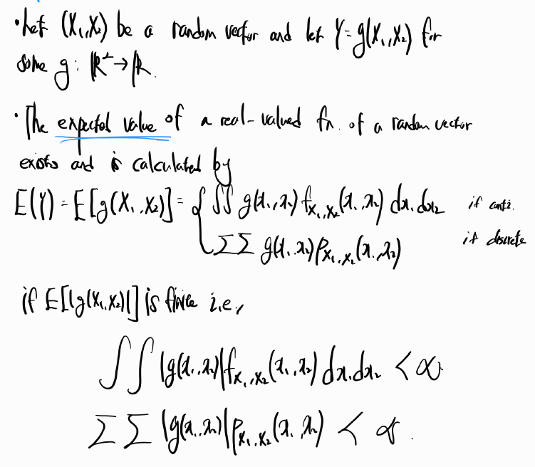
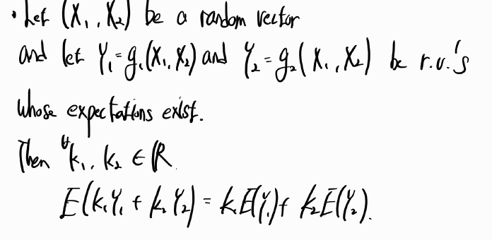
| Expectation of Random Variables (0) | 2024.10.04 |
| Continuous Random Variables (0) | 2024.10.04 |
| Discrete Random Variables (1) | 2024.10.04 |


| Multivariative Distribution - Distributions of Two Random variables (0) | 2024.10.04 |
|---|---|
| Important inequalities (0) | 2024.10.04 |
| Expectation of Random Variables (0) | 2024.10.04 |
| Continuous Random Variables (0) | 2024.10.04 |
| Discrete Random Variables (1) | 2024.10.04 |


| Important inequalities (0) | 2024.10.04 |
|---|---|
| Some special Expectations (0) | 2024.10.04 |
| Continuous Random Variables (0) | 2024.10.04 |
| Discrete Random Variables (1) | 2024.10.04 |
| Random variables (3) | 2024.09.20 |