exestudiary

부족한 영어 실력을 키우고자 학교에서 지원하는 어학연수를 듣고 있습니다. 

문법이 틀리고 어순이 이상할 수 있지만 너그럽게 봐주시면 감사드리겠습니다.

볼드체는 GPT의 힘을 빌린 표현입니다..ㅎㅎ

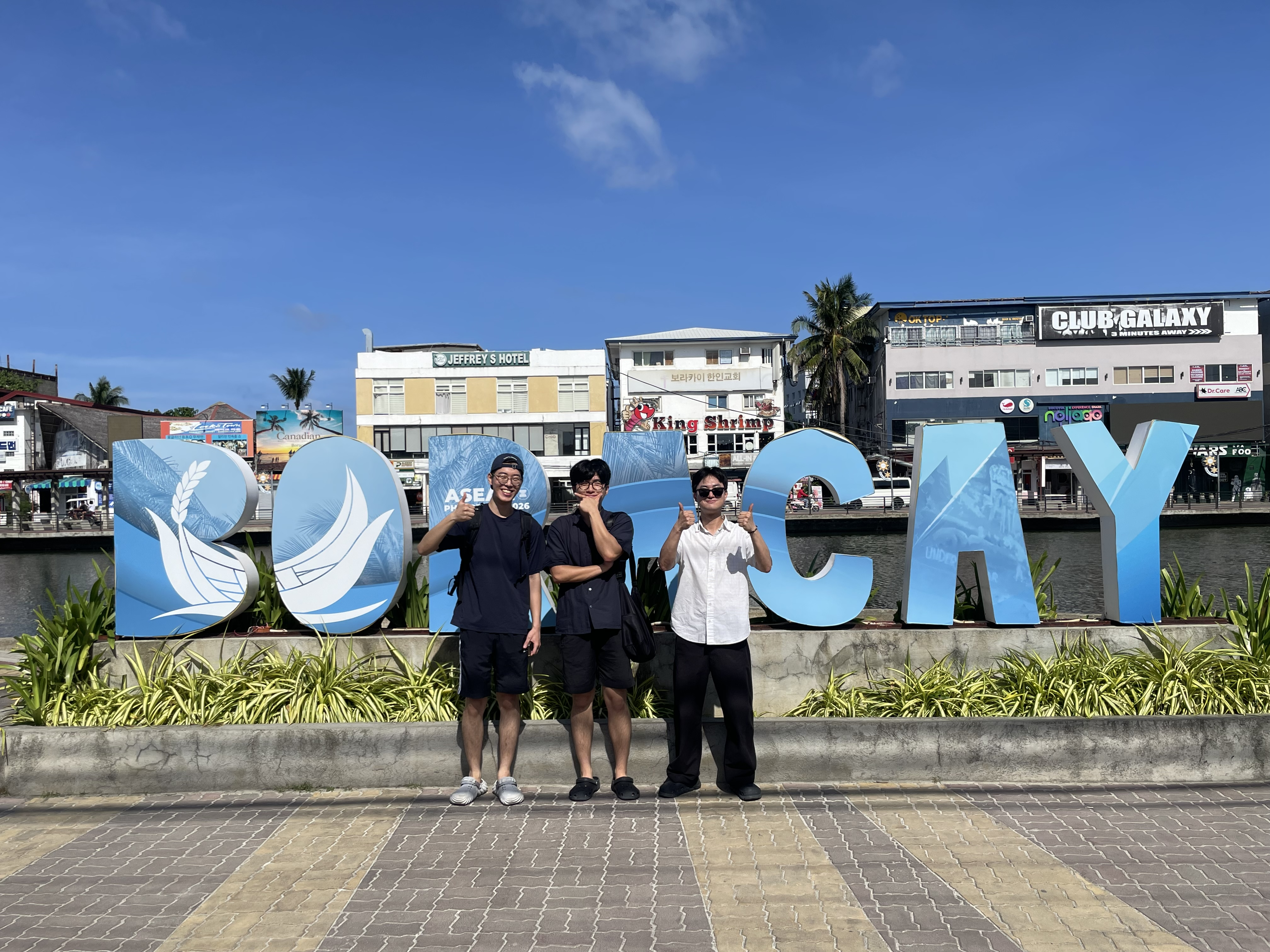
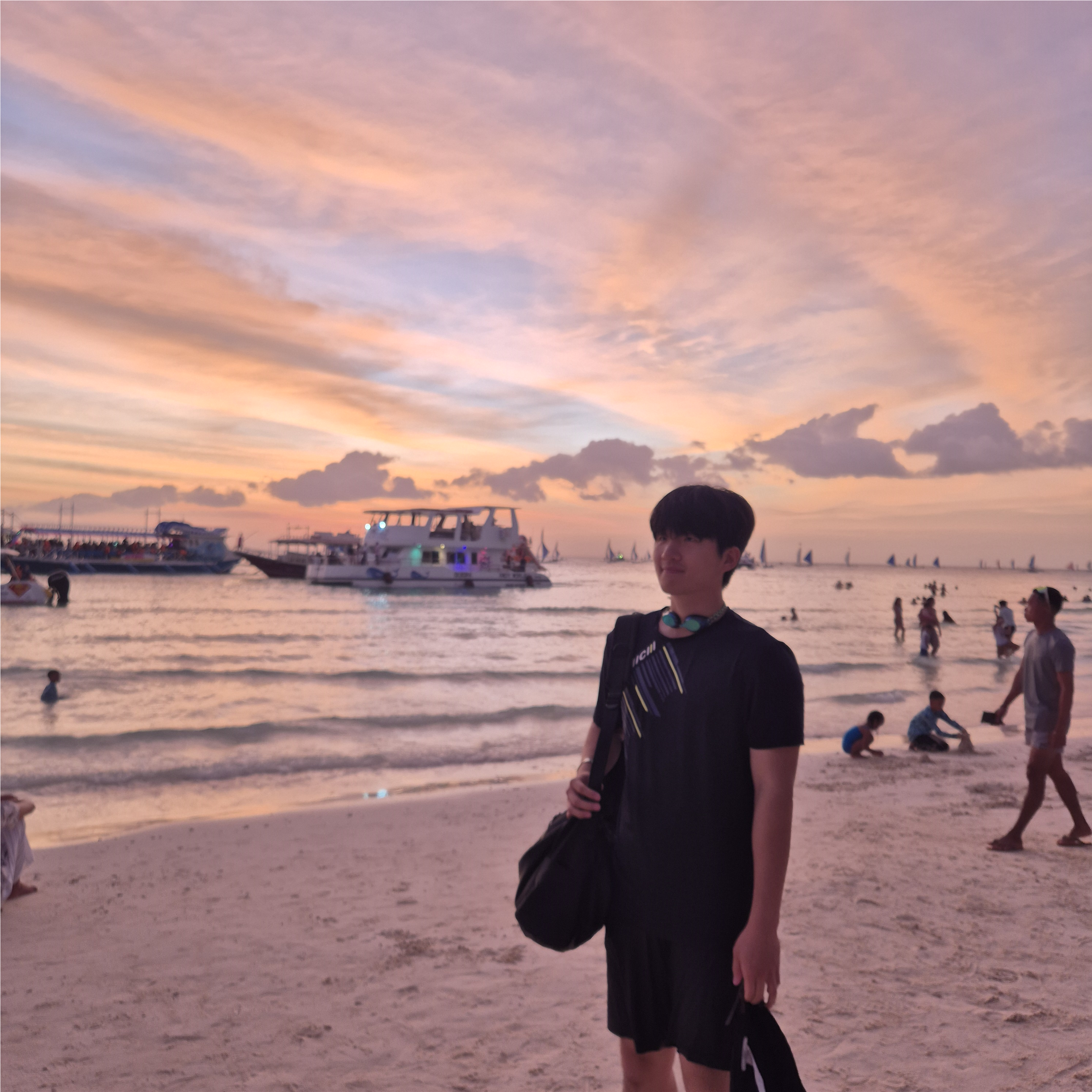
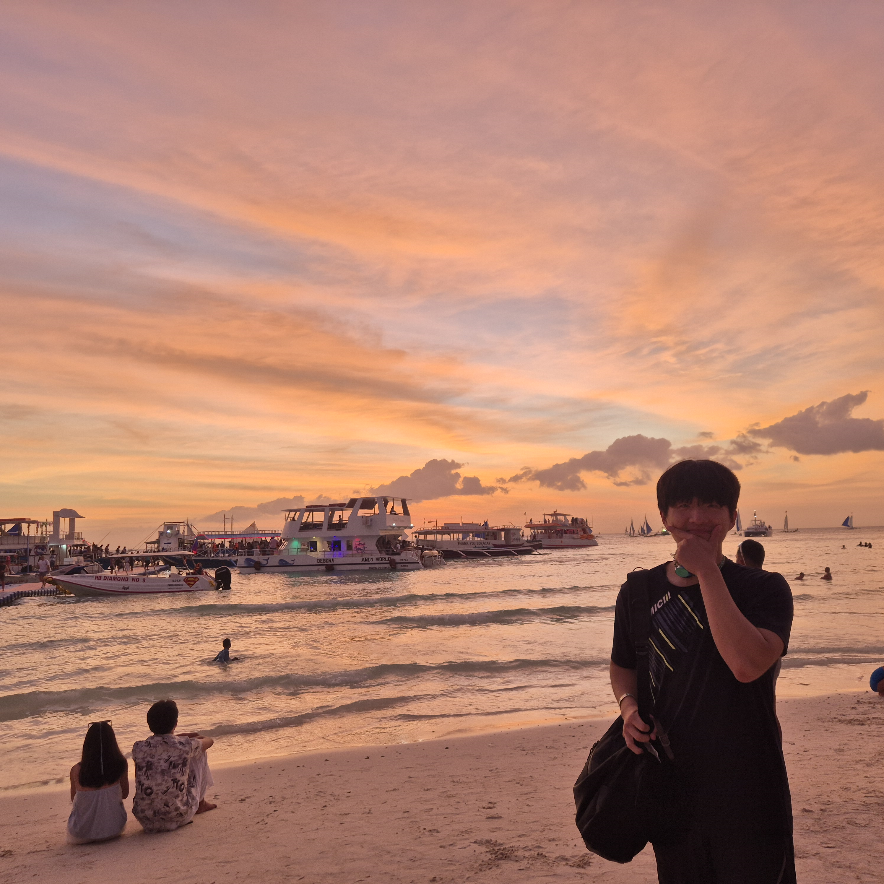
Today I want to talk about my Boracay trip in Philipphines.

It was a very nice trip that I ever went. 

If I have a chance to go there again, I will go there with my GF. 

First day, it was hard to go Boracay. 

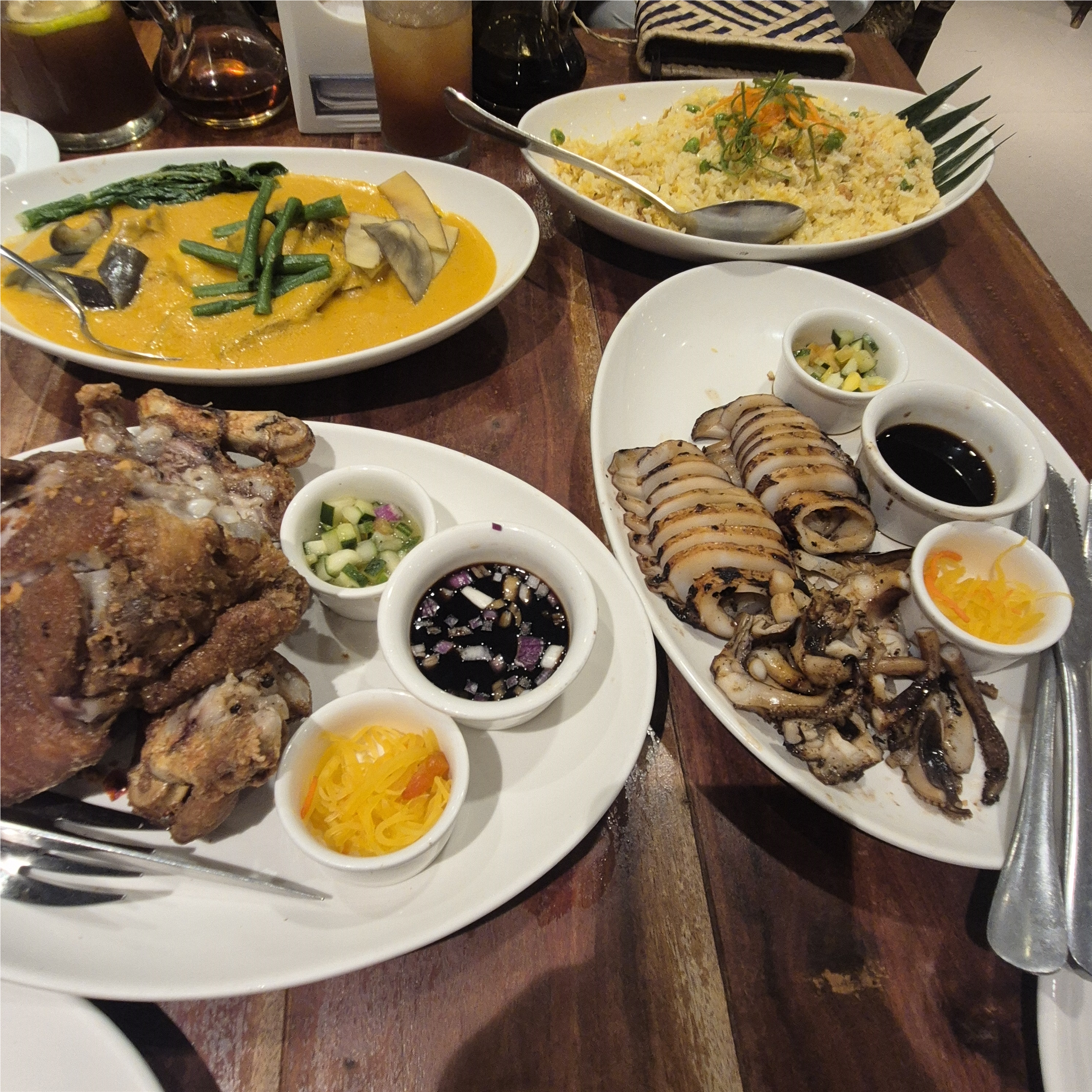
Because we took a bus and ship. Our total time to get there is eleven hours. So, when I arrived in Hotel, I wanted to relax. But, I thought 'If I relaxed, it is a waste of time.' So, we went to Jumbo crab which is famous for crab dishes. 

It was really delicious to eat. But, it was very expensive to pay. I guess why Jumbo crab was so expensive. It's because this resturant is managed by Korean. 

So, we discussed about that "If we have to live in here and manage our business, then can you live in Philipphines whole life?" Then, I said that "I can't live without Kimchi. So, I'm out." But, my friends said "If we get more money with that, I will try that." Yeah.. It's a reasonable answer. But, I experience that it is difficult to live in foreign country even though I have many friends in there. Therefore, nowadays, I think that It is hard to study in U.S.A. Because, you know, the price of U.S.A is more expensive than Korea and Philipphines. So, I am nervous about that. 

Even though It is not confirmed that I can go U.S.A for Doctor's course, I have to be worried about my future. 

There is nothing to confirm. So, to face my future life is scared to me. 

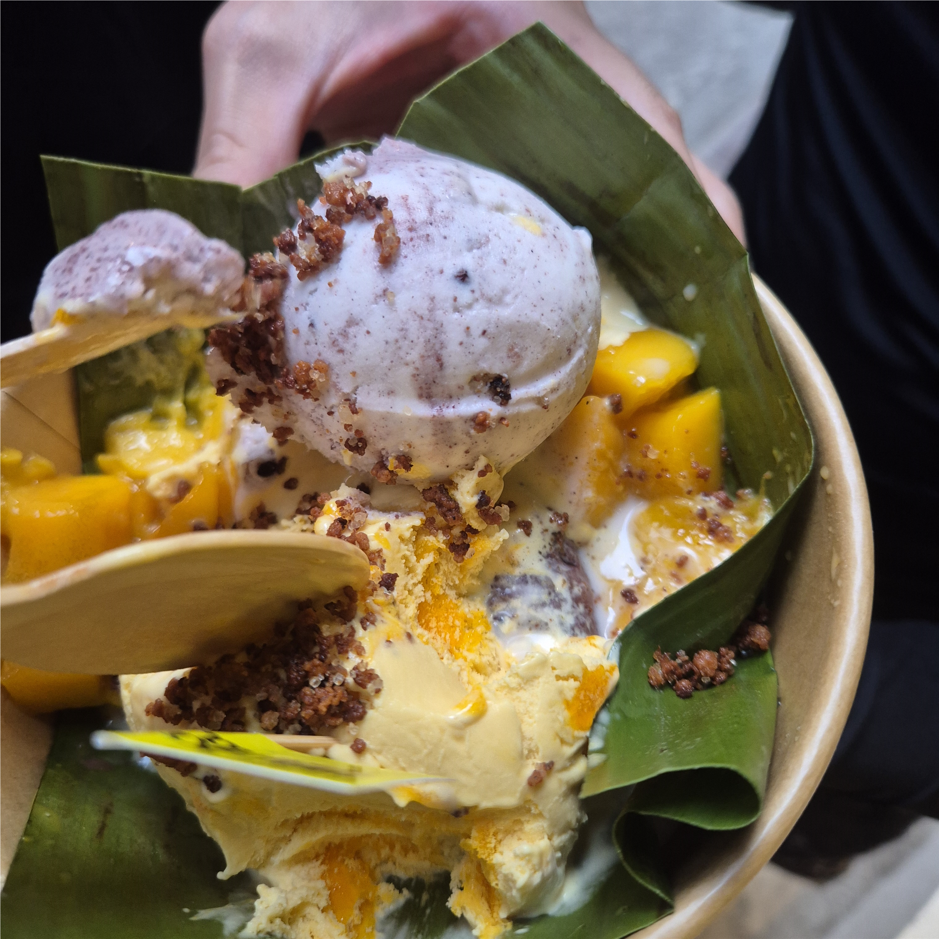
Anyway, I think to write about Boracay trip by Korean is better than to do by English. Because there are many pictures I want to post on my blog. The network of dormitory is not actually good. So, I will come back with Boracay story written by Korean later. 

But, I will write English diary until the rest of the day.

Have a good day!!

부족한 영어 실력을 키우고자 학교에서 지원하는 어학연수를 듣고 있습니다. 

문법이 틀리고 어순이 이상할 수 있지만 너그럽게 봐주시면 감사드리겠습니다.

볼드체는 GPT의 힘을 빌린 표현입니다..ㅎㅎ

When I woke up, I felt my body don't want to go school. 

Because today is Philipphines holiday. So, I really don't want to go to school. 

But, if I endure three days, I can go to Boracay which has many things to play.

So, I went to school. Yeah.. I talked about Korea's situation with my toeic speaking teacher.

She was surprised about our country's atmosphere. She said "I didn't know about the exchange rate about won to dollar."

I said all the things that I know about my nation. And She said to me, "You looks old. But It is nice. Because Young people have to know about what happening in own country."

I also agree with my teacher's saying. 

Anyway, after a class, we went to karaoke with my Korean friends. I really like to sing when I am free from my working or studying. So, I was very happy about that moment. 

Tomorrow, I will stay in dormitory to manage my health before going to Boracay. 

Guys, Take care about your health everyday.

See you!

부족한 영어 실력을 키우고자 학교에서 지원하는 어학연수를 듣고 있습니다. 

문법이 틀리고 어순이 이상할 수 있지만 너그럽게 봐주시면 감사드리겠습니다.

볼드체는 GPT의 힘을 빌린 표현입니다..ㅎㅎ

I went to Lakawon on Saturday.

It was very nice. 

Because the sea and island was so beautiful. 

If I have a chance to go there, I want to go one more time. 

But, after playing, I felt tired. So, as soon as I got in the car, I took a nap. 

Then, when I woke up and turned around to see our group members, they also fell asleep. 

Today I learned some interesting expression. 

1.read between the lines

 > My grandmother is very indirect. I always have to read between the lines to get what she's really saying.

2. spill the beans

 > Don't spill the beans about Anika's surprise party! She can't know about it! 

3. keep a lid on something 

 > The government is trying to keep a lid on prices.

 > Keep a lid on it.

4. get a hold of

 > Did you get a hold of him?

5. get our wires crossed 

 > I think we got our wires crossed.

 > Sorry, we must have gotten our wires crossed.

6. beating around the bushes 

 > Stop beating around the bush.

7. be on the same page

 > We’re on the same page.

8. bite my tongue 

 > She bit her tongue during the meeting.

So, I am gonna use these expression tomorrow. 

Nowadays, I want to read a book. Because it is fun to read between the lines. I am interested about soloving a problem.

Anyway, I have a secret. Don't spill the beans guys. I heard that it is okay to go outside when I go to Boracay. 

Don't get a hold of anyone who don't know this fact. 

부족한 영어 실력을 키우고자 학교에서 지원하는 어학연수를 듣고 있습니다. 

문법이 틀리고 어순이 이상할 수 있지만 너그럽게 봐주시면 감사드리겠습니다.

볼드체는 GPT의 힘을 빌린 표현입니다..ㅎㅎ

Hello! Today, I was fine because of medicine.

So, I decided to go outsied to play basketball with filiphino friends. 

I didn't play well in the last game. So, I wanted to play well in this game. 

My three point shot was goal. So, I felt it was nice start. After that, I also shot the ball when I get the second chance. I got the goal. So, I thought, 'My hand is hot. So, I have to let my teammate pass me the ball.' 

But, it was the last goal in the game. LOL.

I was sad about that my performance wasn't well. 

So, now I think I have to play basketball when I come back to my country. 

To remind my past basketball skill, practicing is important.

Oh, and nowadays, I learn American English pronunciation by Duolingo. 

I want to know the director of Duolingo. Because UI is very comfortable to use.

So, I can see my rank within people who use Duolingo. 

Also, I can get new phrase and expression by it. 

After using this app, I get to know that learning English regularly is important than going another country to learn English.

I think I will learn English by Duolingo when I come back to Korea.

Today, I feel that it is important to use money with plan as I pay my money in Phlilppine. 

I have to use money with plan when I come back to Korea. 

Thank you for reading. 

And Tomorrow I will go Rakawon which is coast. 

I am very excited to go there. 

Because I endure my desire to drink for this moment. 

I also write diary after the trip. 

So, coming soon!

필리핀 어학연수에서 재미로 만들어 본 이력서입니다!

그렇게 많은 커리어가 현재 있지는 않지만 나날이 더 많이 채워 가보겠습니다.

감사합니다.

pdf

부족한 영어 실력을 키우고자 학교에서 지원하는 어학연수를 듣고 있습니다. 

문법이 틀리고 어순이 이상할 수 있지만 너그럽게 봐주시면 감사드리겠습니다.

볼드체는 GPT의 힘을 빌린 표현입니다..ㅎㅎ

Long time no see. 

I was sick at Wednesday and Thursday. 

So, I couldn't write my diary. 

My diagnostic name is a traveler's diarrhea. It means when traveler drinks foreign water, colon bacillus can live in my stomach. So, I had a headache before lunch.

Also, I did a speech contest. I think I prepared well. But, I didn't get a prize. 

I just got the certificate of participation. I was shocked by the result. Because, even though I had a mistake, I spoke pretty well. So, I think it is reasonable to anticipate that I can get the prize. 

But, I didn't. So, I was very depressed about the result of speech contest. 

Because I memorized all things of scription and I got some compliment about speech. 

Well,,, I don't care about the speech, now. The one thing that I can focus on is to improve my english communication skills. 

I am sick little now, too. So, I can't write more than this. 

Oh.. anyway, I will post my resume soon. 

Thank you for reading my diary.

부족한 영어 실력을 키우고자 학교에서 지원하는 어학연수를 듣고 있습니다. 

문법이 틀리고 어순이 이상할 수 있지만 너그럽게 봐주시면 감사드리겠습니다.

볼드체는 GPT의 힘을 빌린 표현입니다..ㅎㅎ

Today, I prepared my resume and draft of speech contest scription.

It was fun for me because when I arrange my experience, I feel proud myself. 

There are many prizes in my career. So, I also bragged to my group mates. 

My teacher said, "You are already hired." It means that you have many careers so, it is weird if company do not hire me. 

Yeah... Actually, I think so too. 

But, I think in my major's friends also have many careers. For example, the tallest guy in our master's course already worked in public institution. And then he has more prizes than me. 

I think he can be a salary man if he apply to some big company.

Everytime I see him, I think that "why he is in Kyungpook National University?"

Even though KNU is Korea No.1 University, it is true that KNU is not competitve in the present than in the past.

So, I always respect to what he did. And I also try my best to chase his career. 

And he is also humble. 

I think he is already ready for getting a new job. 

Hmm... It seems like I've been talking only about my friend. 

Oh! I also work out at the gym. 

When I exercised with my friends, the gym manager came to us and said "Can I take your photo and post on a instagram?" 

We said "Yes!" 

And here's the photo and link about his gym. 

I think It is cheapest gym in the Bacolod.

If you are interested in Learning English program in Bacolod and working out, come this Gym.

Thank you for reading.

And I will come back tomorrow!

부족한 영어 실력을 키우고자 학교에서 지원하는 어학연수를 듣고 있습니다. 

문법이 틀리고 어순이 이상할 수 있지만 너그럽게 봐주시면 감사드리겠습니다.

볼드체는 GPT의 힘을 빌린 표현입니다..ㅎㅎ

I decided to register in a speech contest. 

I wasn't supposed to take part in contest. But, I think this is the last chance to do presentation in front of audience. 

So, after a lot of thought, I decided to do it.

But, when I heard about the prize. I was little bit regretful because the prize is Khan's spa which I visited yesterday. 

Wow.... I can get three Khan's spa coupon if I win the contest. 

Actually, I am not pressured. But, My teacher Joyce said "you can do it. Don't feel pressured about getting the prize. It is a chance to improve your English communication."

I'm really grateful because my teacher always encourages me.

Then, Anyway, I want to talk about what I learned today.

There are many expressions and vocabulary.

balance: staying equal

athletic: being good at sports

pierced: small horn on the skin

muscular: having big and strong muscles.

cosmetics: make up

beard: under the lips.

irrestible: hard to say "no"

trim: cut a little

plastic surgery: medical surgery to change or improve how someone looks

mustache: upper the lips.

dress up

> The restaurant is pretty fancy, so you'll need to dress up.

drop by

> Why don't you drop by some time this weekend so you can see my new kitten?

fall through

> Anne was devastated when her wedding plans to Richard fell through, but two years later she married someone much better suited to her. 

get along 

> Monica and Walid don't get along at all. I can't invited them both to my dinner party, or there will be dramal.

get by

> New York is expensive, so it's hard to get by there with a low-paying job.

That's all I learned today.

I felt stuck. Because there are many words that I don't know yet. 

You know, I like to figure things out as I go.

So, there are many things that I have to do. Like preparing for contest, doing homework, studying English by using GPT or DuoLingo. 

I got some feeling that "Am I good, now?" during studying English recently.

I can't feel that I develope my English skills. 

Sometimes I understand English less than I did on the first day.

But as always, I believe that change is happening little by little within me.  

So, I am gonna trust myself. 

Thank you for reading! 

부족한 영어 실력을 키우고자 학교에서 지원하는 어학연수를 듣고 있습니다. 

문법이 틀리고 어순이 이상할 수 있지만 너그럽게 봐주시면 감사드리겠습니다.

볼드체는 GPT의 힘을 빌린 표현입니다..ㅎㅎ

Today, I went to church with Korean friends.

It was good. Because Fillipino welcomed us.

Since I arrived in the Philippines, I feel they really love Korean. 

It's nice. But, sometimes it feels like pressure to me. 

Because they are very active.

Like this, people in the church also sing a song actively. 

And there were many children. 

On the other hand, I admired that kind of energy. You know, children in Korea decrease every year. 

So, I can't see that kind of energy anymore in my hometown. 

The thing is, the country can be powerful when we make place where children can play.

Anyway, I was exhausted because of the powerful Sunday worship. 

To take a different kind of rest, we went to massage shop.

We paid 400 peso per person. 

It was good. But, when massage therapist massaged my head, it was very painful. 

She pulled the hair along the sides off my face. 

So, I was not satisfied with that massage shop. 

Next time, I am going to go hotel massage shop. Maybe, It would be greater than before shop.

And then, I went to cafe with two Korean friends. 

I met my Fillipion's friend who play basketball with me on the way to cafe.

He gave ball to me. But, I couldn't score in one try. 

So, I decided to buy my basketball to practice everyday. Tomorrow I will go SM town.

Yeah,, Today was a normal day. 

I'm sure that there are many events tomorrow. 

So, that's it for today's diary. 

Thank you for reading.

And I will come back with interesting story. 

1. I'm trying to ~ (I'm trying to sleep.)
2. I'm supposed to ~ (I'm supposed to be there now.)
3. I was about to ~ (I was about to call you.)
4. I'm here to ~ (I'm here to help you.)
5. I've been ~ing (I've been waiting for you.)
6. Let me ~ (Let me check.)
7. Can I get ~ (Can I get a coffee?)
8. Can you ~ ? (Can you help me?)
9. Do you mind ~ing? (Do you mind opening the window?)
10. I'm not sure if~ (I'm not sure if it works.)
11. I don't think ~ (I don't think that it's true.)
12. I think you should ~ (I think you should try it.)
13. It feels like ~ (It feels like summer.)
14. It looks like ~ (It looks like rain.)
15. It sounds like ~ (It sounds like a plan.)
16. There is / There are ~ (There is a problem.)
17. I'd like to ~ (I'd like to order now.)
18. I need you to ~ (I need you to wait.)
19. I just wanted to ~ (I just wanted to say thank you.)
20. I was wondering if ~ (I was wondering if you could help.)
21. The thing is ~ (The thing is, I'm busy today.)
22. As far as I know ~ (As far as I know, he left.)
23. You don't have to ~ (You don't have to worry.)
24. You might want to ~ (You might want to check again.)
25. It depends on ~ (It depends on the situation.)
26. I'll let you know ~ (I'll let you know later.)
27. I didn't mean to ~ (I didn't mean to hurt you.)
28. I can't wait to ~ (I can't wait to see you.)
29. That's why ~ (That's why I left early.)
30. That's what I mean. (That's what I mean.)