exestudiary

(학부생이라 오류가 있을 수 있습니다. 댓글로 정정해서 남겨주시면 감사드리겠습니다.)

단순선형회귀는 input이 하나이고 이 input을 통해 y값을 예측하는 모형입니다.

input이 만약에 여러 개면 Mutiple linear regression이라고 하는데 이 부분은 다음 포스팅 때 다뤄보도록 하겠습니다.

단순선형회귀는 독립변수 하나와 종속변수의 관계를 관측할 수 있게 해주는 설명력이 높은 통계적 방법입니다. 

회귀분석의 첫 단추를 끼우는 만큼 단순선형회귀에 대해 제가 배운 내용을 바탕으로 설명을 해보겠습니다. 

Simple linear regression model

• The response variable $Y$ 와 the predictor variable $X$ 는 $$ Y = \beta_0 + \beta_1X + \epsilon $$, where $\epsilon$ is a random error with $E(\epsilon) = 0$. (Population 수준의 모델)

Simple regression model with the observed data

• The regression model for the observed data is $$ y_i = \beta_0 +\beta_1x_i + \epsilon_i,   i = 1, 2, ...., n$$, where $\epsilon_i$ represents the error in $y_i$.

Parameter estimation

• To estimate the unknown regression coefficients, $\beta_0$ and $\beta_1$, the ordinary least squares(OLS) method is commonly used. 
• From the regression model, we can write $$\epsilon_i = y_i - \beta_0 - \beta_1x_i,  i = 1, 2,.... , n.$$
• We estimate $\beta_0$ and $\beta_1$ by minimizing $$ S(\beta_0, \beta_1) = \displaystyle\sum_{i=1}^{n}{(y_i - \beta_0 - \beta_1x_1)^2}$$ >> 가장 오른쪽에 있는 식은 Convex function이어서 미분 최솟값 구하면 됩니다.  

우리가 parameter 값을 구하고 싶은데, 현실은 observed data의 X와 Y값 만을 알고 있는 상태입니다. 

그렇기 때문에 우리는 parameter 값을 추정하는 겁니다.  실제 X값과 Y값을 통해 구할 수 있는데,

추정은 다음과 같은 식을 통해 구할 수 있습니다. 

OLS estimate 

• It can be shown that the estimates of \beta_0 and \beta_1 that minimize $S(\beta_0, \beta_1)$ are given by $$\hat{\beta_1} =  \frac{\sum_{i = 1}^{n}{(y_i - \overline{y})(x_i - \overline{x})}}{\sum_{i = 1}^{n}{(x_i - \overline{x})^2}}$$ and $$ \hat{\beta_0} = \overline{y} -  \hat{\beta_1}\overline{x}$$
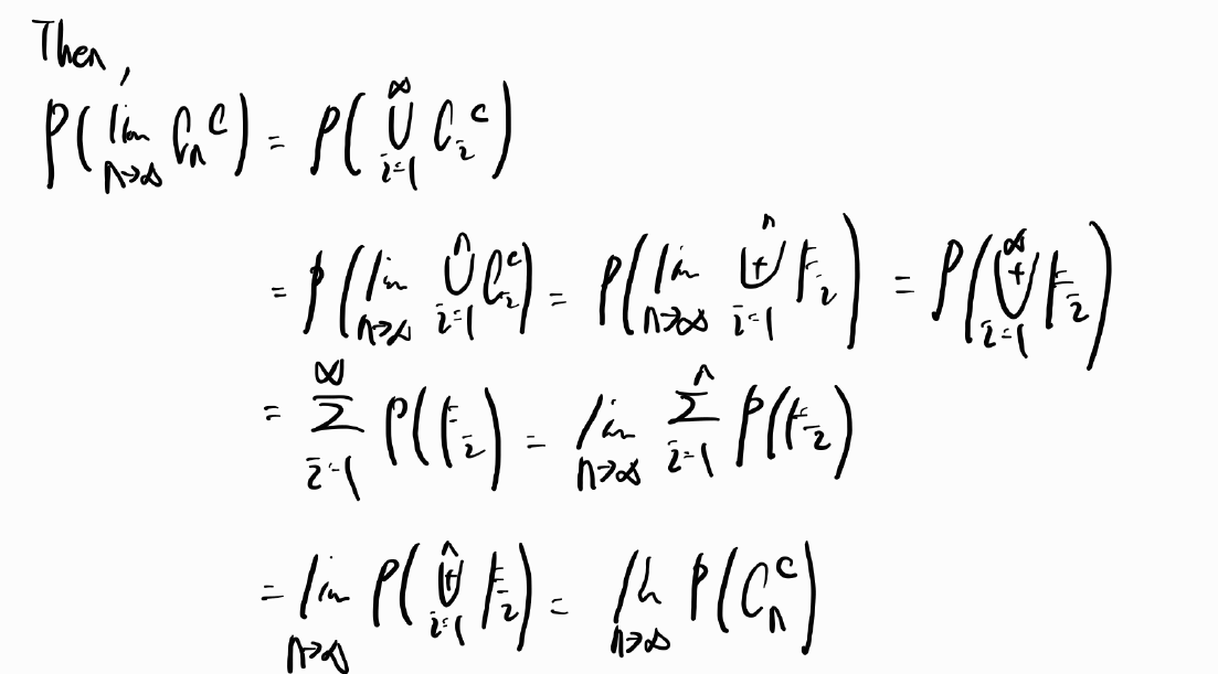
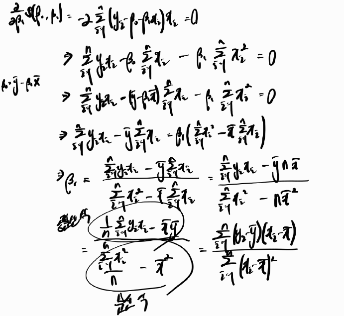
• $ \hat{\beta_0} = \overline{y} -  \hat{\beta_1}\overline{x}$ 증명

• $\hat{\beta_1} =  \frac{\sum_{i = 1}^{n}{(y_i - \overline{y})(x_i - \overline{x})}}{\sum_{i = 1}^{n}{(x_i - \overline{x})^2}}$ 증명

이렇게 하여 $\hat{\beta_0}$ 과 $\hat{\beta_1}$을 구할 수 있는데,

여기서 $\hat{}$ 을 취한 이유는 True 값(추정치가 아닌 값)을 모르고 추정치만 알고 있어서 $\hat{}$을 취했습니다.

Fitted values

• The OLS regression line is obtained as $$ \hat{Y} = \hat{\beta_0} + \hat{\beta_1}X $$.
• The $i$-th fitted value is given by $$ \hat{y_i} = \hat{\beta_0} + \hat{\beta_1}x_i,  i = 1, 2, ..., n$$.
• Example.

이렇게 fitted 했다면 해석은 어떻게 해야 하는지 궁금할 수 있을 것 같은데요... 

그런데 그 전에 $ Y = \beta_0 + \beta_1X + \epsilon $ 이 식 양변에 평균을 취하게 되면 다음과 같이 나옵니다.

$$ E(Y) = \beta_0 + \beta_1X$$.

왜 이렇게 나오냐면 $E(\beta_0 + \beta_1X + \epsilon)$ 에서 $ \beta_0 + \beta_1X $는 이미 값을 알고 있고 그렇기 때문에 상수로 처리됩니다. 그러면 자연스럽게 $ \beta_0 + \beta_1X  + E(\epsilon)$ 이 되고, 회귀분석에서는 $E(\epsilon) = 0$이라고 하는 아주 중요한 가정이 있기에 자연스럽게 $E(Y) = \beta_0 + \beta_1X$ 이 식이 유도가 됩니다. 

Interpertation of coefficients

• Recall that $$ E(Y) = \beta_0 + \beta_1X$$.
  - $\beta_0$ is the expected value of $Y$ when $X = 0$.
  - $\beta_1$ is the amount of increase in the expected value of $Y$ for every one-unit increase inn $X$.
• For example E(minutes) = 4.162 + 15.509 $\times$ Units.
  - The average length of calls is the 4.162 minutes when no component needs to be repaired.
  - The average length of calls increases by 15.509 minutes for each additional component that has to be repaired. 

Test of hypothesis

• In the simple linear regression analysis, the usefulness of the predictor(= X) can be tested by using the following hypothesis test:
  $H_0: \beta_1 = 0   versus   H_1: \beta_1 \neq 0$.
  (X와 Y의 linear relationship을 $\beta_1$을 체크하여 확인할 수 있습니다.)
  (주의할 점: $\hat{\beta_1}$을 이용해서 가설검정을 하는 것이 아닙니다.)
• To this end, we need to further assume that
  
  

이렇게 간단한 식에 4가지의 가정이 들어가있습니다. 중요하기에 반드시 알아두는게 좋다고 합니다.

1. $E(\epsilon_i) = 0$

2. $Var(\epsilon_i) = \sigma^2$

3. $\epsilon_i$ ~ Normal

4. $\epsilon_1, ..... \epsilon_n$ are independent.

T-test

• Under $H_0$ : $\beta_1 = 0$, it can be shown that $$ T = \frac{\hat{\beta_1}}{s.e.(\hat{\beta_1})}$$ follows a Student's t distribution with n - 2 degrees of freedom, where $$ s.e.(\hat{\beta_1}) = \sqrt{\frac{\sum_{i=1}^{n}{(y_i - \hat{y_i})^2/(n-2)}}{\sum_{i=1}^{n}{(x_i - \overline{x})^2}}}$$.

Using t-distribution, we can compute the p-value. At significant level $\alpha = 0.05$, we reject $H_0$ if the p-value $\leq$ 0.05. Otherwise, we fail to reject $H_0$.

보통은 모델이 유용하기를 바라기 때문에 귀무가설을 기각하기를 원합니다. 

앞서말한 계수들 뿐만 아니라 $\sigma^2$를 추정하는 것도 중요한데요

바로 error의 변동성을 설명하기 위함입니다.

Estimation of $\sigma^2$

• Define $$ e_i = y_i - \hat{y_i}, i = 1, 2, .... , n $$ which are called the residuals.
  이렇게 하는 이유는 $\epsilon_i = y_i - \beta_0 - \beta_1x_i$를 
• We can estimate $\sigma^2$ by using $$ \hat{\sigma^2} = \frac{\sum_{i=1}^{n}{e_i^2}}{n - 2} = \frac{\sum_{i=1}{n}{(y_i - \hat{y_i})^2}}{n-2} \equiv $$ MSE, 
  where $\sum_{i=1}{n}{(y_i - \hat{y_i})^2}$ is referred to as SSE (Sum of Squares of Errors) and n -2 is called the df(degrees of freedom).
  여기서 n은 전체 데이터이고 2는 추정치의 개수입니다. 추정치는 $\beta_0, \beta_1$으로 2개가 존재했습니다. 그렇기에 2를 빼주는 것입니다. 

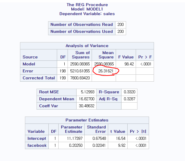
SAS라는 통계 프로그램을 통해서 MSE를 관측할 수 있는데 밑에 그림의 빨간색 부분이 MSE입니다. 

MSE in SAS

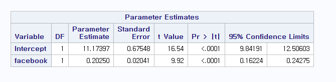
Confidence intervals 

• The (1 - $\alpha$) $\times$ 100% confidence intervals (or limits) for $\beta_0 and \beta_1$ are given by $$ \hat{\beta_0} \pm t_{n-2,\alpha/2} \times s.e.(\hat{\beta_1})$$,
  where $t_{n-2, \alpha/2}$ is the (1 - $\alpha$ / 2) percentile of a t - distribution with n - 2 df

이렇게 신뢰구간도 설정하고 회귀모델을 fitting 했으면 이제 예측을 해봅시다

(예측은 크게 설명력과 예측력으로 구분할 수 있습니다.)

Prediction

• There are two types of predictions:
  1. Prediction of the value of Y given X, i.e., $Y = \beta_0 + \beta_1X + \epsilon$.
  2. Prediction of the mean of Y given X, i.e., $E(Y) = \beta_0 + \beta_1X$.

여기서 하나 알아갈 수 있는 점은 confidence interval은 prediction of the value of Y given X가 넓을 수 밖에 없습니다. 왜냐하면 $\epsilon$, 즉, error가 포함되어 있기 때문입니다. 

• Given $X = x_0$,
  - in the first case, the predicted value is $\hat{y_0} = \hat{\beta_0} + \hat{\beta_1}x_0$.
  - in the second case, the mean response is $\hat{\mu_0} = \hat{\beta_0} + \hat{\beta_1}x_0$.

Prediction intervals

• The (1 - $\alpha$) $\times$ 1000% prediction limits are given by $$\hat{\mu_0} \pm t_{n-2,\alpha/2} \times s.e.(\hat{\mu_0})$$ and $$\hat{y_0} \pm t_{n-2, \alpha/2} \times s.e.(\hat{y_0})$$,
  where $$s.e.(\hat{\mu_0}) = \hat{\sigma}\sqrt{\frac{1}{n} + \frac{(x_0 - \overline{x})^2}{\sum_{i=1}^{n}{(x_i -\overline{x})^2}}}$$ and $$ s.e.(\hat{y_0}) = \hat{\sigma}\sqrt{1+ \frac{1}{n} + \frac{(x_0 - \overline{x})^2}{\sum_{i=1}^{n}{(x_i -\overline{x})^2}}} $$
  
  (여기서 보면 Expected value와 value 값의 interval을 측정할 때 차이점이 보입니다. 바로 1이 더해졌냐 안 더해졌냐인데요. value값은 아까 Prediction 파트에서 value값의 confidence interval이 넓을 수 밖에 없다고 한 것과 비슷한 매락의 이야기입니다. $\sigma^2$은 $\epsilon$의 분산이고 $\epsilon$만큼 더해진 것을 확인할 수 있습니다. 그렇기에 더 넓은 confidence interval을 가질 수 밖에 없다고 설명한 것입니다.)

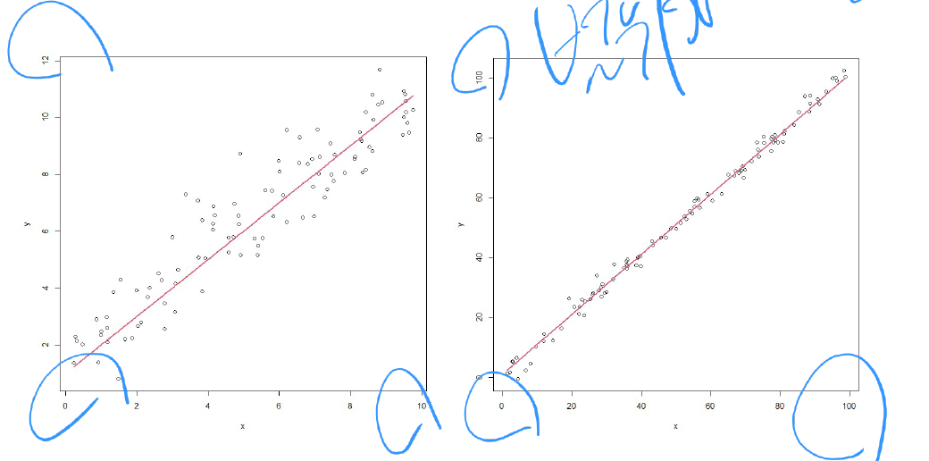
Role of $\sigma^2$

• 분산이 크다는 것은 값들이 선에 비교적 가깝지 않고, 분산이 작다는 것은 선에 비교적 선에 가깝다는 얘기입니다. 
• 그러나 분산 즉, $\sigma$의 분산만을 가지고는 선형성을 추론하기에 어려움이 있습니다. 가령, 범위가 다를 때는 $\sigma$의 분산으로 선형성을 추론하면 오류가 발생할 수 있습니다.

그래서 이 상황에서 고안된 것이

Measuring the strength of the linear relationship

• To remedy the limitation of $\sigma^2$, we can propose to use $$\frac{\sigma^2}{Var(Y)}$$, since it decreases if $\sigma^2$ decreases or $Var(Y)$ increases.
• 우리는 $\sigma^2$의 값을 모르기 때문에 $\sigma^2$의 추정치인 MSE를 사용할 것입니다. 복습을 하자면 $$MSE = \frac{\sum_{i=1}^{n}{(y_i-\hat{y_i})^2}}{n-2}$$ 이고 $Var(Y)$도 모르기 때문에 추정치인 $\hat{Var}(Y)$을 사용할 것입니다. 이것도 다시 remind 하자면 $$ \hat{Var}(Y) = \frac{\sum_{i=1}^{n}{(y_i-\overline{y})^2}}{n-1} $$ 입니다. 

여기서 선형성인 것을 나타내주는 지표인 결정계수가 나옵니다.

$R^2$

• To measure the strength of the linear relationship, we define the so-called $R^2$ as follows:
  $$R^2 = 1 - \frac{\sum_{i=1}{n}{(y_i - \hat{y_i})^2}}{\sum_{i=1}{n}{(y_i-\overline{y})^2}} = 1 - \frac{SSE}{SST}$$
  where SST stands for the total sum of squared deviation in $Y$ from its mean.

Property of $R^2$

• It can be shown that $$\displaystyle\sum_{i=1}^{n}{(y_i - \overline{y})^2} = \displaystyle\sum_{i=1}^{n}{(\hat{y_i}-\overline{y})^2} + \displaystyle\sum_{i=1}^{n}{(y_i - \hat{y_i})^2}$$
  where 왼쪽 식에서 첫 번째 식은 SSR(the sum of squares due to regression)으로 불린다.
  That is, $$SST = SSR + SSE$$.
  
  
• This implies that $$0 \leq R^2 \leq 1$$
  (그 이유는 $R^2  = SSR/SST$ and $0 \leq SSR \leq SST$).

Random variables(확률 변수)

random variable 은 일종의 함수라고 생각하면 된다.

probability space에서 real space(실수 집합)으로 mapping이 된다고 생각하면 된다. 

예를 들어 random variable $ X $를 주사위를 두 번 굴려서 나온 윗 면의 합이라고 하면,

$X(i, j) = i + j$로 나타낼 수 있고 $ X $의 space는 {2, ... 12}가 된다. 

The Sample space는 $ {(i, j) : 1 \leq i, j \leq 6} $이 되고 $ P[{(i, j)}] = 1 / 36 $이다.

즉, 주사위 윗면의 의미로서 1, 2, 3, 4, 5, 6이 X라는 확률변수 함수를 만나서 실수로 표현이 될 수 있다는 것이다.

Probability Mass Function

여기서 앞서 말한 주사위 사례를 들어보자. 

$B_1 = {x : x = 7, 11}$ and $B_2 = {x: x = 2, 3, 12}$ 라고 할 때,

$P_x(B_1) & P_x(B_2)$를 구해보자. 그러면 간단하게 다음과 같이 나타내면 된다. 

Probability Density Function

Choosing a real number at random from (0, 1).

Let $X$ be the number chosen & the space of $ X $ is $ D $(데, space의 개념이다.) = (0, 1).

The pdf of $X$ is $f_X(x) = I_(0 < x < 1)$, where $I_A$ be an indicator function of a set $A$.

E.g. the probability that $X$ is less than an eighth or greater than seven eights is 

$$ P[{X < 1/8} \cup {X > 7/8}] = \int_0^\frac{1}{8} \mathrm{d}x + \int_\frac{7}{8}^1 \mathrm{d}x = \frac{1}{4}$$ 

Cumulative Distribution Function(CDF)

Example 

Suppose we roll a fair die. Let $X$ be the upface of the roll and the space of $X$ is {1, 2, 3, 4, 5, 6}.  

The pmf is $p_X(i) = 1/ 6, i = 1, 2, 3, 4, 5, 6$.

If $x < 1, P(X \leq x) = 0$; If $1 \leq x < 2, P(X \leq x) = p_X(1) = 1 /6$, and so on. 

Hence, the cdf of $X$ is

= 위에 D가 있는 것은 X 와 Y의 확률 변수가 같다는 의미가 아니라 CDF가 같다는 뜻이다. 즉, 분포적 성질이 같다는 것과 같다. 

Theorems

Conditional Probability (조건부 확률)

The probability that $C_2$ occurs given that event $C_1$ has occurred is called the conditional probability of $C_2$ given $C_1$ and is defined by 

그림으로 표현하자면 아래와 같다.

Conditional probability is a probability? 

조건부확률이 확률의 정의를 만족하는지 살펴보자.

Properites of Conditional Probability

Ex. Four cards are to be dealt successively, at random and without replacement, from an ordinary deck of playing cards. The probability of receving a spade, a heart, a diamond, and a club, in that order is.. 

$C_1$ : 1st - 13 / 52

$C_2$ : 2nd - 13 / 51

$C_3$ : 3rd - 13 / 50

$C_4$ : 4th - 13 / 49

(카드 놀이에서 4번을 뽑는데 각각 다른 걸 뽑을 확률을 나타낸 것)

- Prior probability vs. posterior probability

- Let $C_1, ... C_k$ : k causes of an event.

- P($C_i$) indicates the chance of $i$th cause.

  If known, it is obtained from the past investigation >>>> prior probability 

  (쉽게 말해 알려진 확률을 prior probability)

- P($C_i | C$) indicates the chance of $i$th cause when the event $C$ happened.

  It updates the past information >>>> posterior probability

Independence

1. Statistically / stochastically independent means independent in a probability sense.
2. Two events A and B are independent if and only if $P(A|B) = P(A|B^c) = P(A)$ or $P(B|A) =P(B|A^c) = P(B)$. Otherwise, they are independent.
3. Events $C_1, C_2, C_3$  are pairwise independents if and only if $P(C_1 \cap C_2) = P(C_1)P(C_2)$, $P(C_1 \cap C_3) = P(C_1)P(C_3)$, $P(C2 \cap C_3) = P(C_2)P(C_3)$.

Mutual Independence (모든 경우가 독립이면)

ex. Pairwise independence does not imply mutual independence

1,2,3,4가 적혀있는 spinner를 2번 돌렸다. 

$C_1$은 두 번 돌린 spinner의 숫자의 합이 5가 되는 사건이고, $C_2$는 첫 번째 돌렸을 때 1이 나오면 되는 사건이고, $C_3$는 두 번째 돌렸을 때 4가 나오면 되는 사건이다. 

표를 통해서 모든 경우의 수를 생각해보면

$C_1$ > 빨간색

$C_2$ > 파란색

$C_3$ > 민트색

Then $P(C_i) = 1/4, i = 1, 2, 3$, and for $i \neq j$, $P(C_i \cap C_j) = 1/16$.

Thus, C_1, C_2, C_3 are pairwise independent.

But, $C_1 \cap C_2 \cap C_3$ is the event that (1, 4) is spun and its probability is 1/16.

$P(C_1 \cap C_2 \cap C_3) = 1 / 4 \times 1/4 \times 1/4 \neq 1 / 16 $

이것이 의미하는 것이 두 사건이 독립이라고 해서 mutual independence가 성립한다고 보장할 수 없다를 예제를 통해서 확인할 수 있다. 

$\sigma$-field

$ \sigma $ - field는 위의 세 조건을 반드시 만족해야한다. 

Example

1. Find the smallest $\sigma$-field of subsets of $C$(체) = {1, 2, 3}.

2. Find the largest $\sigma$-field of subsets of $C$(체) = {1, 2, 3}.

Probability Space

Theorems 

Remark

Thm 3.6. Continuity Property

위의 특징을 시각화하면 아래의 그림과 같다.

반드시 increasing sequence라는 조건이 있어야 한다.

증명을 해보면

파란색 별 모양이 의미하는 것이 $C_n$이 increasing sequence 중에서 가장 마지막에 나오는 집합이기에 앞서 나온 집합들을 다 포함할 수 있다는 것이다. 그러고 난 다음에 우리는 donut 모양으로 집합을 생각할 것인데 이것은 mutually exclusive의 성질을 사용하여 집합의 덧셈으로 표현하기 위함이다. 아래와 같이 표현할 수있다. 

그러면 mutually exclusive 하기에 다음과 같이 표현이 가능하다.

decreasing sequence의 경우에도 같은 방향으로 살펴볼 수 있다. 그런데 이 때는 여집합을 사용해서 mutually exclusive한 성질을 사용하고자 한다. 

이것이 성립하기 때문에 모든 식에 여집합을 취해주면 증명하고자 하는 식이 도출된다. 

1. Set and Subset

- Set: a collection of objects (elements).

- 어떤 Set $ C_1 $의 모든 element가 $ C_2 $의 element라면 Set $ C_1 $ 은 $ C_2 $의 Subset이라고 한다.

∀ $  x \in C_1 $ , $x \in C_2 $

Denoted by C_1 \subset C_2

Example 

- Define two sets $ C_1 $ = {(x, y) : 0 $\leq$  $x$ = $y$ $\leq$ 1}  and $ C_2 $ = {($x$, $y$) : 0 $\leq$ $x$ $\leq$ 1, 0 $\leq$ $y$ $\leq$ 1}. Because the elements of $ C_1 $ are the points on one diagonal of the square, then $C_1 \subset C_2 $. 

- Remark: $C_1 = C_2$  <=> $ C_1 \subset C_2$ & $C_2 \subset C_1 $

2. Intersection 

- Intersection: $ C_1 \cap C_2 $ (= {$x$ | $x \in C_1$ and $ x \in C_2$})

집합이 유한개: 

집합이 무한개: 

- Null set: $ C = \emptyset $

If $ C_1 \cap C_2 = \emptyset $, then $C_1$ and $C_2$ are said to be mutually exclusive or disjoint.

3. Union

- Union: $C_1 \cup C_2$ (= {x | $ x \in C_1$ or $ x \in C_2 $})

- (Notation) 

- 집합의 수에 따라 나눈 것(위: 유한개, 아래: 무한개)

4. Space and Complement

여기서 보면 Space의 표기가 다르다는 것을 확인할 수 있다. ('체'나 '데' 라고 부른다고 한다.)

5. Useful Algebra

Commutative Laws(교환법칙), Associative Laws(결합법칙), Distributive Laws(분배법칙), DeMorgan's Laws(드모르간의 법칙)

6. Point functions

1.  $f(x) = 2x, -\infty$ $ < x < $ $ \infty $
2. $$g(x, y) =\begin{cases} {e}^{-x-y},\;  \; 0 < x < \infty,\ 0 < y < \infty \\ 0,\; \; elsewhere \end{cases}$$
3. $$h(x_1,...,x_n) = \begin{cases} 3x_1 \cdots x_n, \; \; 0 \leq x_i \leq 1, i = 1, 2, \ldots, n \\ 0, \; \; elsewhere \end {cases}$$

Point function은 Point가 input되고 하나의 값이 도출된다는 것을 의미한다. 

7. Set functions

Let $C$ be a set in two-dimensional space and 

$$Q(C) = \begin{cases} the \ area \ of \ C, \;\; C \ has \ a \ finite \ area \\ undefined, \;\; otherwise \end{cases}$$ 

1. $$ C = {(x, y) : x^2 + y^2 \leq 1} \to Q(C) = \pi \times 1^2 = \pi$$
2. $$ C = {(0, 0), (1, 1), (0, 1)} \to Q(C) = 0 + 0 + 0 = 0 $$
   1. 점의 넓이는 0이기에 0 + 0 + 0 이다.
3. $$ C = {(x, y) : 0 \leq x, 0 \leq y, x + y \leq 1} \to Q(C) = \frac{1}{2}$$ 

1. Experiment (실험)

- Any action or process by which observations (or measurements) are generated.

- The only way in which an investigator can elicit information about any phenomenon is to perform the experiments.

- Each experiment terminates with an outcome.

- If an experiment can be repeated under the same conditions, it is called a random experiment.

2. Sample space $ S $ (표본 공간 $ S $) 

- The sample space is a set that contains all possible outcomes of a particular experiment.

• The number of outcomes in the sample space can be finite or infinite.
• Infinite sample space can be countable or uncountable. A sample space is countable if the elements of the sample space can be put into 1-1 correspondence with a subset of the integers.

3. Event (사건)

- An event of a sample space $ S $ is a subset of $ S $ (including $ S $ itself).

• A simple event contains only one outcome. Denoted by $ w $.
• A compound event contains two or more outcomes.

4. Probability (Relative Frequency Approach)

- Suppose that an experiment is performed N times.

- The relative frequency for an event A is $ A occurs \over N $  = $ f \over N $.

- If we let N get infinitely large, $$ P(A) = lim_{N\to\infty}{f_N \over N}$$