x1 = 5 ; x2 = 7
x1+x2
y = x2 - x1
ls() # 현재 저장된 변수 리스트 확인
rm(y) ; ls() # y만 삭제 후 변수 리스트 확인
rm(list = ls()) ; ls() # 저장된 변수 모두 삭제 후 변수 리스트 확인
변수의 종류
numeric(수치형)
character(문자형)
logical(논리형)
complex(복소수형)
저장된 변수의 자료형 확인
mode(x1) # numeric으로 출력
str(x1) # num 5로 출력
is.numeric(x1) # numeric 외에 자료형 다 가능
변수의 자료형 변경
as.numeric(x1) # as.character(x1)
# 연습
num1 =  1; char1 = 'a' ; logi1 = T

is.numeric(num1) # T
is.character(logi1) # F
is.logical(char1) # F

as.numeric(logi1)
as.character(num1)
as.logical(char1) # NA, character의 경우 logical로 바꿀 수 없음.
file_hander = open("output.txt", "wt", encoding = "utf-8")

while True:
    words = input("Enter words >>> ")
    if word.startswith("exit"):
    	break

    else:
    	file_handler.write(words)

file_hander.close()
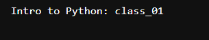
입력파일 확인
파일에서 한 칸씩 띄워서 넣고 싶을 때
file_hander = open("output_1.txt", 'wt', encoding = "utf-8")

while True:
	words = input("Enter words >>> ")
    if words.startswith("exit"):
    	break

    else:
    	file_handler.write(words)
        file_handler.write("\n")

file_hander.close()
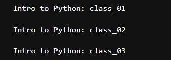
파일 확인
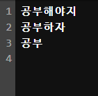
마지막에 4줄까지 표시가 된 것은 공부를 입력하고 file_handler.write("\n")을 통해 한 줄이 띄워진 것이다.
writelines() 함수
words_list = \
['안녕하세요.', 'Python', '잘하고 싶은 사람입니다.'] # \는 라인이 길어서 두 줄로 표현했다는 뜻

with open("output.txt", "wt", encoding="utf-8") as fp:
    fp.write("\n".join(words_list)) # join은 리스트를 하나의 문자로 만들어주는데 그것의 연결고리가 \n이 되도록
    fp.flush()
# 각각의 원소의 결과값을 알기 위해 실행하는 코드
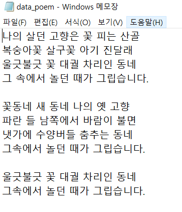
file_example = open("data.txt", "rt")
line_list = file_example.readlines()
for line in line_list:
print(line)
file_example.close()
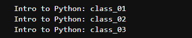
이렇게 출력되는데 이것은 print가 default값으로 \n을 가지기 때문이다.
이걸 해결해주기 위해 다음과 같은 코드를 짤 수 있다.
# 각각의 원소의 결과값을 알기 위해 실행하는 코드
file_example = open("data.txt", "rt")

line_list = file_example.readlines()

for line in line_list:
	line = line.strip("\n")
	print(line)

file_example.close()
mat = matrix(1:10, nr = 5)

cbind(mat, c(1:5)+3)
cbind(c(1:5)+3, mat)
cbind(mat, c(1:5)+3, c(1:5)-3) # 순서대로 저장됨.
cbind(c(1:5)+3, mat, c(1:5)-3)
# cbind 설명
# Take a sequence of vector, matrix or data-frame arguments and combine by columns.
data.frame
paste("id", 10) # 입력한 2개의 문자를 띄어쓰기써서 붙여주기
paste0("id", 10) # 입력한 2개의 문자를 띄어쓰기없이 붙여주기

example3 = example[sample(1:nrow(example), 10), 1:5] #여기서 example은 전에 썼던 파일 (covid)
new = paste0("id", 1:nrow(example3))

#### add variable(1) ----
cbind(example3, new)
cbind(new, example3)

#### add variable(2) ----
example3$id = new
example3[, c("id", "age", "gender","occupation", "line_of_work", "time_bp")]
example3[,c("age", "id", "gender", "occupation", "line_of_work", "time_bp")]
기준에 따라 inner join, outer join, left join, right join
inner / outer
left / right
예제
df1 = data.frame(
    ID = 1:6,
    group = c(rep("B",3), rep("A",2), "B")
)

df2 = data.frame(ID = 3:7, score =c(31,86,76,83,53))

## merge 사용 ----

# inner join
merge(df1, df2) #merge(df1, df2, by ="ID")

# outer join
merge(df1, df2, all = TRUE)

# left join
merge(df1, df2, all.x = TRUE)

# right join
merge(df1, df2, all.y = TRUE)

# 중복되는 변수가 존재하는 경우(값이 완전히 동일)
df3 = data.frame(ID=3:5, score=c(31, 86, 76))
merge(df2, df3, by="ID") # score.x와 score.y가 나옴.
merge(df2, df3, by="ID")[,c("ID","score.x")]
Practice
# mtcars의 자료에 k-번째 관찰값이면 'car_k' 값을 가지는 변수 id를 맨 앞에 추가하여 cars로 저장
cars = cbind(id = paste0("car", nrow(mtcars)), mtcars)

# cars 자료 중에 1~10번째 관찰값을 추출하고 변수 id, mpg, disp만 cars1으로 저장
cars1 = cars[1:10, c("id","mpg","disp")]

# cars 자료 중 '1~5번째 관찰값'과 '6번째 이후 관찰값에 대하여 랜덤으로 추출한 5개의 관찰값'에 대하여
# 변수 id, mpg, cyl만 cars2로 저장
cars2 = cars[c(1:5, sample(6:nrow(cars), size = 5)), c("id","mpg","disp")]

# 함수 merge를 활용하여 변수 id를 기준으로 cars1, cars2에 대하여 inner join/ left join/ outer join
merge(cars1, cars2, by = "id")
merge(cars1, cars2, by = "id", all.x = TRUE)
merge(cars1, cars2, by = "id", all = TRUE)
# 내장 데이터 iris3 불러오기
data(iris3)

# iris3의 데이터 구조 파악하기
str(iris3)

# iris3의 세 번째 페이지의 행의 수 구하기
nrow(iris[,,3])

# iris3의 세 번째 페이지의 변수 Sepal L.의 분산 구하기
var(iris3[,"Sepal L.",3])

# 값 "A", "B", "C"를 중복 허락하여 iris3의 세 번째 페이지의 행의 수만큼 추출한 벡터 label 생성하기
label = sample(c("A", "B", "C")nrow(iri3[,,3]), replace = True)
### install readxl ----
install.packages("readxl")
library(readxl)

### loading excel ----
read_xlsx("C:\\Users\\user\\OneDrive - 경북대학교\\통계학과\\1-2\\R프로그래밍 및 실험\\w5_1 covid19_psyco.xlsx")

read_xlsx("C:\\Users\\user\\OneDrive - 경북대학교\\통계학과\\1-2\\R프로그래밍 및 실험\\w5_1 covid19_psyco.xlsx", col_names = T)

readxl:: read_excel("C:\\Users\\user\\OneDrive - 경북대학교\\통계학과\\1-2\\R프로그래밍 및 실험\\w5_1 covid19_psyco.xlsx", sheet = 2)

readxl:: read_excel("C:\\Users\\user\\OneDrive - 경북대학교\\통계학과\\1-2\\R프로그래밍 및 실험\\w5_1 covid19_psyco.xlsx", na = "NA")

readxl:: read_excel("C:\\Users\\user\\OneDrive - 경북대학교\\통계학과\\1-2\\R프로그래밍 및 실험\\w5_1 covid19_psyco.xlsx", na = "7")
csv 파일로 불러오는걸 선호하기 때문에 csv파일로 불러오는 걸 공부하겠음.
csv
setwd("C:\\Users\\user\\OneDrive - 경북대학교\\통계학과\\1-2\\R프로그래밍 및 실험")
# 내가 어디 폴더에서 파일을 가지고 작업을 수행할지 정해줌.
# 자기 파일 클릭하고 우클릭하면 속성이 있는데 거기서 파일이 어딨는지 정보가 있으니
# 그걸 복사 붙여넣기하면 됨.
# 근데 처음에 복사하면 \ 가 한 개만 나오는데
# \를 \\이렇게 만들어줘야함.

temp = read.csv("w5_1 covid19_psyco.csv", header =FALSE)
# 파일 불러오기
# header는 column_names를 변수로 쓸건지 아닌지 FALSE는 안 쓴다는거
str(temp)
head(temp, n = 5)
tail(temp)
temp$X ; temp$travel.work
unique(temp$age)
10 %in% temp$time_dp
5:10 %in% temp$time_dp
5:10 %in% head(temp$time_dp)

# temp에서 temp$X, temp$travel.work 열을 제거한 데이터 프레임 example 생성하기
example = temp[, -c(20,22)]
example = temp[, !(names(temp) %in% c("X", "travel.work"))]
example = subset(temp, select = -c(X, travel.work))
# temp의 변수 age 내 오타를 수정하고 확인
temp[temp$age == "Dec-18"] == "12-18"

# na개수
sum(is.na(temp$X))
sum(is.na(temp$travel.work))

# na개수와 temp의 행의 수가 같은지 확인
sum(is.na(temp$X)) == nrow(temp)
sum(is.na(temp$travel.work)) == nrow(temp)
Practice2
names(temp)
# 를 통해서 X와 travel.work이 column의 몇 번째인지 알아보기

example = temp[,-c(20,22)]
example = temp[,!(names(temp) %in% c("X", "travel.work")]
exmaple = subset(temp, select = -c(X, travel.work))

# subset(x, select,...)
## x : object to be subsetted
## select : expression, indicating columns to select from a dataframe
### 여기서 select 안에 있는 column의 변수들은 "" 표시 X
파일 내보내기
setwd("C:\\Users\\user\\OneDrive - 경북대학교\\통계학과\\1-2\\R프로그래밍 및 실험")

result = table(example$age, example$prefer)
# age가 행 부분이 되고, prefer이 열 부분이 됨.

write.csv(result, file = "table.csv")
# result라는 데이터 프레임을 csv로 저장
write.csv(table(example$age, example$prefer), file = "table2.csv")

write.csv(example[1:3, 1:4], file = "dataframe.csv")
# example의 1부터 3부분의 행과 1부터 4의 열을 추출해서 csv 파일로 만들고 파일 이름은 dataframe.csv
리스트 저장하기
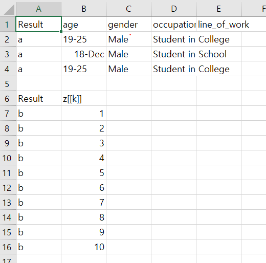
write.csv(list(a = example[1:10, 1:4], b = 1:10),
          file = "list1.csv")
이런 식으로 저장됨.
write.csv(list(a = example[1:10, 1:4], b = 1:5),
		file = "list2.csv")
1번째 데이터 프레임과 2번째 데이터 프레임의 F열 값이 다르다는 것을 확인할 수 있음.
이게 왜냐면
write.csv(list(a = example[1:10, 1:4], b = 1:10),
          file = "list1.csv")
write.csv(list(a = example[1:10, 1:4], b = 1:5),
		file = "list2.csv")
10개의 행을 불러오는건 둘 다 같은데, b의 값이 1부터 10까지인거랑 b가 1부터 5까지인 것에서 차이가 난다는 걸 확인할 수 있음.
### rdata
setwd("C:\\Users\\user\\OneDrive - 경북대학교\\통계학과\\1-2\\R프로그래밍 및 실험")
save(result, file = "rda file.rda")
# save(result, file = "rda file.rdata")
# R의 고유한 저장형식
# 현재까지 작업한 환경을 현 작업공간(working directory)에 저장함.

save.image(file = "image.rda")
# 현재 작업 중인 공간 전체를 저장
load("image.rda")
load("rda file.rda")
# "로드"는 외부 파일에 저장된 데이터나 객체를 R 프로그램에서 사용할 수 있도록 가져오는 과정